Act 14: Pattern Recognition

In this activity, we extract patterns from a given image using image processing in order to define a set of features that will allow us to separate the the set into classes, and to find the most suitable classifier for the task, since some objects can have similar parameters. This prompts us to search for other parameters that may be unique. We take the mean of the numerical values of each of these parameters, and we then compare each object's parameter to the respective mean parameter. For an object to belong to a certain class, their parameter should be close to the mean.

We make use of an assembly of three different kinds of bird seeds: small round seeds, white squash seeds and large reddish-brown seed.

The parameters that were took into account were the size of the seeds and their red color channel values. The graph below summarizes the objects parameter's qualities:

The red colored dot stands for the mean value of the small round seed, the blue for the white squash seed and the blue for the large reddish-brown seed. It can be seen that similar objects are clustered together, save for a few deviations in color, which is between the class of the small round seeds and the white squash seeds. The color discrepancy may be attributed to the uneven illumination of the objects when the image was taken. However, the sizes of the two smaller seeds are somehow distinct from each other, so we can still infer the class the correctly belong to. The largest seeds are very far apart from the other two classes in terms of size, so the somehow large deviations from the mean does not matter.

I will give myself a grade of 10/10 for this activity since the code has successfully classified the objects. I would like to thank Earl for his assistance in data collection and help in the code.

Act 13: Correcting Geometric Distortion

In this activity, we correct a barrel distortion in a given image, in this case a grid, using two methods: bilinear interpolation and nearest neighbor method. The image to be reconstructed is shown below:

We compare the image with an ideal grid constructed computationally in Scilab, which shall serve as the reference image.

The vertices of the grid will serve as reference points for the reconstruction. Firstly, the most undistorted image was located from the image, and the number of pixels down and across one box was counted. For each box, c1 to c8 was computed from the four corner points of the box, which is given by the equation below.

which is in matrix-vector notation

Since we are looking for the coefficients, we manipulate the above equation to

We then determine the location of those points in the ideal rectangle using


The locations of the distorted image were found using Scilab's locate function. The results were also rounded off so that they become integer-valued.

Using nearest neighbor method, the reconstructed image looks like this:

while using bilinear interpolation yields the image below.

As expected, the bilinear interpolation has better quality as compared to the grid reconstructed using nearest neighbor method.

For this activity, I will give myself a grade of 10/10 for accomplishing this activity. I would like to thank Gilbert for his tremendous help in this activity.

Act 12: Color Image Segmentation

In this activity, we try to single out a particular region in a given image by taking a cropped image of the region's surface, and implement it using both parametric segmentation and non-parametric segmentation methods and compare their outcomes. We make use of the image below:

Our region of interest is from that of the silver mouse:

Applying parametric segmentation on the original image using the above region of interest, we get the image below:

As said in the the activity manual, histogram backprojection is similar to what was done in Activity 4, except that the lookup histogram is now two-dimenstional. Thus for the nonparametric part, the following histograms were obtained from the p(r) and p(g) values of the ROI:

Applying histogram backprojection yields the result below


This time, we make use of a portion of the wooden table as a region of interest:

Using parametric segmentation:

The histogram for the nonparametric segmentation is shown below

And the resulting image from histogram backprojection is:

Note that the histograms above correspond properly to the normalized color chromaticity space shown below. The silver mouse appears much more bluish looking and shinier, hence it being closer to both the white and blue regions of the color chromaticity space. On the other hand, the wood ROI, while not exactly white, appears in a region where the colors mix.

It can be seen from the images that the parametric segmentation makes the region of interest much more visible. However, the nonparametric segmentation somewhat recovers specular reflection, as can be seen in both images. Parametric segmentation is more useful when you need to clearly outline the parts of the image that correspond to your region of interest. Nonparametric segmentation may be more useful for manipulating your image, such as changing the regions of interest's colors, hue, brightness, etc.

I will give myself a grade of 8/10 for this activity, due to having finished the exercise. The reduced grade is for not completely understanding the exercise. Hopefully, it will all be explained in the next meeting. I would like to thank Gilbert for helping me with the code in this exercise.

Act 11: Color Image Processing

In this activity, we intentionally take two wrongly balanced images and apply two types of algorithms to properly balance them: the white patch and gray world algorithm.

The first image is an ensemble of colorful objects:

Applying the white patch algorithm:

Applying the gray world algorithm:

For this image it seems better to use the gray world algorithm; the white patch-rendered image seems too bright and oversaturated. The gray world-rendered image seems more natural compared to the former. This is due to the fact that the gray world takes the average of all the colors in the image, and there seems to be a good balance of colors in the assembled ensemble of objects.

For the next image, we make use of an image with different hues of green

The image below is rendered using the white patch algorithm:

The image below is rendered using the gray world algorithm:

For this case it seems better to use the white patch algorithm since the color saturation of the color green actually messes up the overall average color of the image. The color balance of the gray world image as a result is worse than the original.

I will give myself a grade of 8/10 for this activity for somehow being able to accomplish a good part of this activity, but I am hard pressed for time to take images that are set-up in other lighting conditions. I would like to thank Earl for his cooperative work on this activity as well as Rommel for helping me with setting up the objects for the image.

Act 10: Preprocessing Text

In this activity, we use the given Untitled_0001.jpg and crop a portion from it. I chose this particular segment

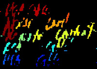
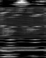
The image was binarized so that it can be processed, and titled by using mogrify so that the lines become horizontal. Performing FFT on the tilted image yields the image for the frequency domain

We can make an appropriate mask to for the above image. I made use of

The masked frequency domain image was returned to the spacial domain using ifft, yielding the image

By applying the appropriate threshold, the image is binarized

Using the closing operator with structural element of a 4x1 matrix consisting of ones, i.e. [1; 1; 1; ], the image below was obtained

Using bwlabel, we can mark the blobs


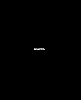
For the last part of the activity, we are to find all the instances of the word 'DESCRIPTION' in the Untitled_0001.jpg. We apply the same routine used in Template Matching using Correlation section of Activity 5. We start by rotating the image using mogrify so that the image is in its proper orientation. We also crop a part of the image containing the word description and place it in a black background with the same size as the original image, like so

Again, we use the same routine as Activity 5, where we apply fft2 on both images. We the correlate the above image with the binarized and rotated Untitled_0001.jpg. The algorithm yields the image below:

It can be seen from the image that there are three white spots. Looking back at Untitled_0001.jpg, the spots appear at the locations of the word 'DESCRIPTION'. Thus, we can say that there are three instances where the word appears.

I've tried to implement an algorithm for automatically checking for the number of instances the word appears in the image. I made use of a for loop to check the the whole normalized image element per element for values sufficiently close to 1, and count them. Fortunately, a value of 3 instances was returned. Unfortunately, I have yet to check if those 3 actually correspond to the correlations. I'll try to get back at this problem sometime later.

For this activity I will give myself a grade of 8/10 since the final processed image seems rougher than I'd want (i.e. the handwriting isn't exactly 1-pixel thick), but I have properly done the last part. I would like to thank Earl for the helpful discussions, and Mimie for teaching me how to properly use bwlabel in tandem with jetcolormap in imshow.

Act 9: Binary Operations

In this activity, we make use of the image below:

And determine the average size of the punched holes. First, we segment the image into a number of parts, which in my case was 9, and we set aside one of those images. I used the image below:

The image is used to determine the saturation level appropriate for the whole image in order to binarize the image and to be able to apply the closing operator. The closing operator works by first eroding the image, then dilating it with a structural element. The structural element I used was

which was a binarized cropped image of a punched hole from the image. This allowed the punched holes to somehow “normalize” to their proper size especially if the image does not seem to form a circle, and if possible, allow sufficiently close holes to separate themselves from each other. It was found that the image had an an average hole size of 512, and thus the code is now useable for the other cropped images. By using bwlabel to label the circles, the area of each circle in an image can be computed. The obtained values are tabulated below:

The histogram is plotted below:

The extremely large values can be attributed to the large accumulation of holes which unfortunately was not resolved by the closing operator. It is difficult to resolve overlapping holes since they sometimes do not exhibit a clear border. By limiting the allowable areas to 400 < x < 600 which is the realistic range of areas for a hole, the average was found to be 504 (503.904762).

I will give myself a grade of 9/10 for being able to completely accomplish all the tasks in this exercise. The reduced grade is for the somewhat large area values resulting from my processing, which I feel could be much better. Again, I would like to thank Earl for the discussions and Gilbert for his help in making a histogram for the areas.

Act 8: Morphological Operations

In this activity, we investigate the effects of the morphological operations erode and dilate when used on an image. We use the following images in particular:

We make use of the following structuring elements on all images for both dilation and erosion operation:
a) 4x4 matrix
b) 2x4 matrix
c) 4x2 matrix
d) a cross 5 pixel long and 1 pixel thick

The images from left to right displayed below will correspond to a to d.
Square
Dilation:

Erosion:



Triangle:
Dilation:

Erosion:



Circle:
Dilation:

Erosion:



Hollow Square:
Dilation:

Erosion:


Cross:
Dilation:

Erosion:


What happens during dilation is that the image expands in the form of the structural element. An example is when the square is dilated using the cross structural element, the square not only expands but its shape also becomes crosslike. Erosion works similarly to dilation, except that it shrinks the image in its form. For example, the hollow square simply becomes four small squares that are positioned in each of the original hollow square's corners.

My submitted predictions were generally correct for the dilation part. Erosion was much harder to predict for me for the triangle, hollow square and cross due to their somewhat irregular shape.

I would grade myself a 9/10 for this activity for being able to perform the operations correctly and a few correct predictions. I would like to thank Earl for his help in this activity.